Robust Soft Learning Vector Quantization¶

A RSLVQ model can be constructed by initializing RslvqModel with the desired hyper-parameters, e.g. the number of prototypes, and the initial positions of the prototypes and then calling the RslvqModel.fit function with the input data. The resulting model will contain the learned prototype positions and prototype labels which can be retrieved as properties w_ and c_w_. Classifications of new data can be made via the predict function, which computes the Euclidean distances of the input data to all prototypes and returns the label of the respective closest prototypes.

Placing the prototypes is done by optimizing the following cost function, called the Robust Soft Learning Vector Quantization (RSLVQ) cost function [1]:

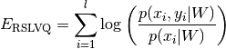
$\displaystyle E_{\mathrm{RSLVQ}} = \sum_{i=1}^l \mathrm{log}\left(\frac{p(x_i,y_i|W)}{p(x_i|W)}\right)$

where $p(x_i,y_i|W)$ is the probability density that $x_i$ is generated by a mixture component of the correct class $y_i$ and $p(x_i|W)$ is the total probability density of $x_i$ .

The optimization is performed via a limited-memory version of the Broyden-Fletcher-Goldfarb-Shanno algorithm. Regarding runtime, the cost function can be computed in linear time with respect to the data points: For each data point, we need to compute the distances to all prototypes, compute the fraction 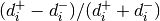$(d^+_i - d^-_i) / (d^+_i + d^-_i)$ and then sum up all these fractions, the same goes for the derivative. Thus, GLVQ scales linearly with the number of data points.

Matrix Robust Soft Learning Vector Quantization (MRSLQV)¶

Matrix Robust Soft Learning Vector Quantization (MRSLQV) generalizes over RSLVQ by learning a full linear transformation matrix $\Omega$ to support classification. The matrix product $\Omega^T \cdot \Omega$ is called the positive semi-definite relevance matrix $\Lambda$ . Interpreted this way, MRSLQV is a metric learning algorithm. It is also possible to initialize the MrslvqModel by setting the dim parameter to an integer less than the data dimensionality, in which case $\Omega$ will have only dim rows, performing an implicit dimensionality reduction. This variant is called Limited Rank Matrix LVQ or LiRaM-LVQ [4]. After initializing the MrslvqModel and calling the fit function on your data set, the learned $\Omega$ matrix can be retrieved via the attribute omega_.

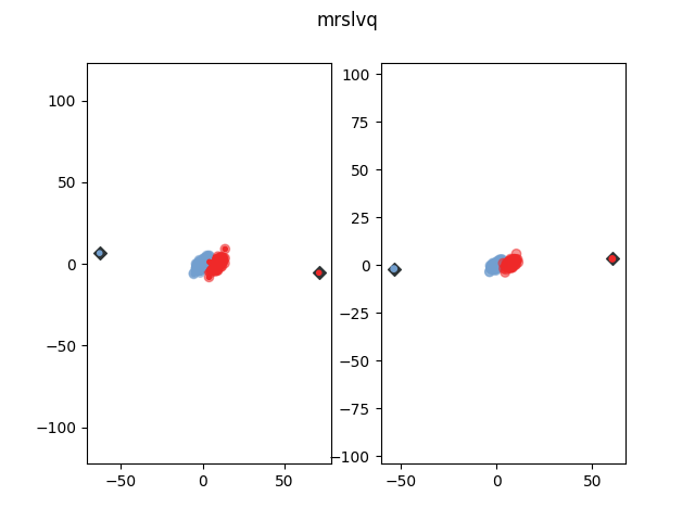
The following figure shows how MRSLVQ classifies some example data after training. The blue dots show represent the prototype. The yellow and purple dots are the data points. The bigger transparent circle represent the target value and the smaller circle the predicted target value. The right side plot shows the data and prototypes multiplied with the learned $\Omega$ matrix. As can be seen, MRSLVQ effectively projects the data onto a one-dimensinal line such that both classes are well distinguished.

References:

[4]	“Limited Rank Matrix Learning - Discriminative Dimension Reduction and Visualization” K. Bunte, P. Schneider, B. Hammer, F.-M. Schleif, T. Villmann and M. Biehl - Neural Networks, vol. 26, nb. 4, pp. 159-173, 2012.

Local Matrix Robust Soft Learning Vector Quantization (LMRSLVQ)¶

LmrslvqModel extends RSLVQ by giving each prototype/class relevances for each feature. This way LMRSLVQ is able to project the data for better classification.

Especially in multi-class data sets, the ideal projection $\Omega$ may be different for each class, or even each prototype. Localized Matrix Robust Soft Learning Vector Quantization (LGMLVQ) accounts for this locality dependence by learning an individual $\Omega_k$ for each prototype k [1]. As with MRSLVQ, the rank of $\Omega$ can be bounded by using the dim parameter. After initializing the LmrslvqModel and calling the fit function on your data set, the learned $\Omega_k$ matrices can be retrieved via the attribute omegas_.

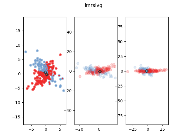
The following figure shows how LMRSLVQ classifies some example data after training. The blue dots show represent the prototype. The yellow and purple dots are the data points. The bigger transparent circle represent the target value and the smaller circle the predicted target value. The plot in the middle and on the right show the data and prototypes after multiplication with the $\Omega_1$ and $\Omega_2$ matrix respectively. As can be seen, both prototypes project the data onto one dimension, but they choose orthogonal projection dimensions, such that the data of the respective own class is close while the other class gets dispersed, thereby enhancing classification accuracy. A MrslvqModel can not solve this classification problem, because no global $\Omega$ can enhance the classification significantly.

References:

[1]	(1, 2) “Distance Learning in Discriminative Vector Quantization” Petra Schneider and Michael Biehl and Barbara Hammer - Neural Computation, pp. 2942-2969, 2009.