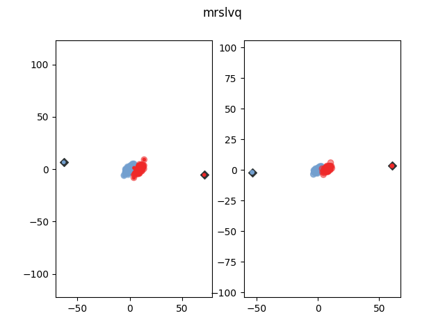
Matrix Robust Soft Learning Vector Quantization

This example shows the different glvq algorithms and how they project different data sets. The data sets are chosen to show the strength of each algorithm. Each plot shows for each data point which class it belongs to (big circle) and which class it was classified to (smaller circle). It also shows the prototypes (light blue circle). The projected data is shown in the right plot.

Out:

MRSLVQ:
('classification accuracy:', 1.0)
('variance coverd by projection:', 100.0)

import numpy as np
import matplotlib.pyplot as plt

from sklearn_lvq import MrslvqModel
from sklearn_lvq.utils import plot2d

print(__doc__)

nb_ppc = 100
toy_label = np.append(np.zeros(nb_ppc), np.ones(nb_ppc), axis=0)

print('MRSLVQ:')
toy_data = np.append(
    np.random.multivariate_normal([0, 0], np.array([[5, 4], [4, 6]]),
                                  size=nb_ppc),
    np.random.multivariate_normal([9, 0], np.array([[5, 4], [4, 6]]),
                                  size=nb_ppc), axis=0)
mrslvq = MrslvqModel(sigma=1)
mrslvq.fit(toy_data, toy_label)

print('classification accuracy:', mrslvq.score(toy_data, toy_label))
#mrslvq.omega_ = np.asarray([[1,-0.11587113],[-0.11597687,0]])
plot2d(mrslvq, toy_data, toy_label, 1, 'mrslvq')
plt.show()

Total running time of the script: ( 0 minutes 2.377 seconds)