Generalized Learning Vector Quantization¶

A GLVQ model can be constructed by initializing GlvqModel with the desired hyper-parameters, e.g. the number of prototypes, and the initial positions of the prototypes and then calling the GlvqModel.fit function with the input data. The resulting model will contain the learned prototype positions and prototype labels which can be retrieved as properties w_ and c_w_. Classifications of new data can be made via the predict function, which computes the Euclidean distances of the input data to all prototypes and returns the label of the respective closest prototypes.

Placing the prototypes is done by optimizing the following cost function, called the Generalized Learning Vector Quantization (GLVQ) cost function [2]:

$\displaystyle E_{\mathrm{GLVQ}} = \sum_{i=1}^l \Phi\left(\frac{d^+_i - d^-_i}{d^+_i + d^-_i}\right)$

where $d^+_i$ is the squared Euclidean distance of $x_i$ to the closest prototype $w_k$ with the same label $(y_i = c_k)$ and $d^-_i$ is the squared Euclidean distance of $x_i$ to the closest prototype w_k with a different label $(y_i \neq c_k)$ . Note that an LVQ model will classify a data point correctly if and only if $d^+_i < d^-_i$ , which makes the cost function a coarse approximation of the classification error.

The optimization is performed via a limited-memory version of the Broyden-Fletcher-Goldfarb-Shanno algorithm. Regarding runtime, the cost function can be computed in linear time with respect to the data points: For each data point, we need to compute the distances to all prototypes, compute the fraction 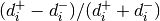$(d^+_i - d^-_i) / (d^+_i + d^-_i)$ and then sum up all these fractions, the same goes for the derivative. Thus, GLVQ scales linearly with the number of data points.

References:

[2]	“Generalized learning vector quantization.” Sato, Atsushi, and Keiji Yamada - Advances in neural information processing systems 8, pp. 423-429, 1996.

Generalized Relevance Learning Vector Quantization (GRLVQ)¶

In most classification tasks, some features are more discriminative than others. Generalized Relevance Learning Vector Quantization (GRLVQ) accounts for that by weighting each feature j with a relevance weight $\lambda_j$ , such that all relevances are $\geq 0$ and sum up to 1. The relevances are optimized using LBFGS on the same cost function mentioned above, just with respect to the relevance terms. Beyond enhanced classification accuracy, the relevance weights obtained by GRLVQ can also be used to obtain a dimensionality reduction by throwing out features with low (or zero) relevance. After initializing a GrlvqModel and calling the fit function with your data set, you can retrieve the learned relevances via the attribute lambda_.

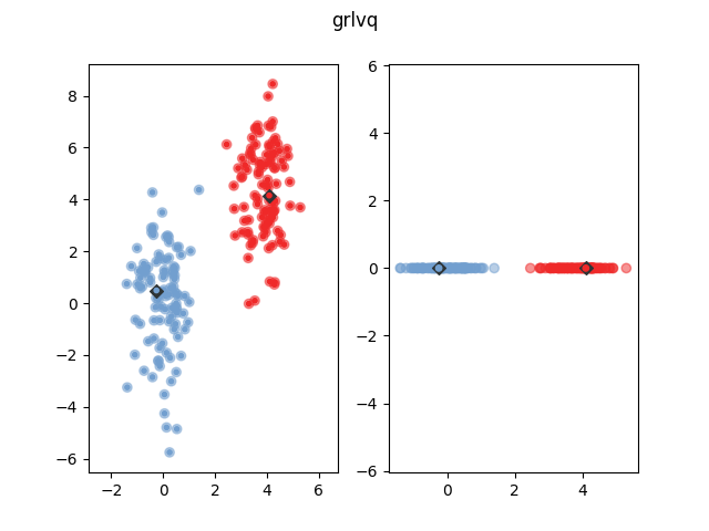
The following figure shows how GRLVQ classifies some example data after training. The blue dots show represent the prototype. The yellow and purple dots are the data points. The bigger transparent circle represent the target value and the smaller circle the predicted target value. The right side plot shows the data and prototypes multiplied with the feature relevances. As can be seen, GRLVQ correctly dismisses the second dimension, which is non-discriminative, and emphasizes the first dimension, which is sufficient for class discrimination.

References:

“Generalized relevance learning vector quantization” B. Hammer and T. Villmann - Neural Networks, 15, 1059-1068, 2002.

Generalized Matrix Learning Vector Quantization (GMLVQ)¶

Generalized Matrix Learning Vector Quantization (GMLVQ) generalizes over GRLVQ by not only weighting features but learning a full linear transformation matrix $\Omega$ to support classification. Equivalently, this matrix $\Omega$ can be seen as a distortion of the Euclidean distance in order to make data points from the same class look more similar and data points from different classes look more dissimilar, via the following equation:

$||\Omega \cdot x_i - \Omega \cdot w_k||^2 = (\Omega \cdot x_i - \Omega \cdot w_k)^T \cdot (\Omega \cdot x_i - \Omega \cdot w_k) = (x_i - w_k)^T \cdot \Omega^T \cdot \Omega \cdot (x_i - w_k)$

The matrix product $\Omega^T \cdot \Omega$ is also called the positive semi-definite relevance matrix $\Lambda$ . Interpreted this way, GMLVQ is a metric learning algorithm [3]. It is also possible to initialize the GmlvqModel by setting the dim parameter to an integer less than the data dimensionality, in which case Omega will have only dim rows, performing an implicit dimensionality reduction. This variant is called Limited Rank Matrix LVQ or LiRaM-LVQ [4]. After initializing the GmlvqModel and calling the fit function on your data set, the learned $\Omega$ matrix can be retrieved via the attribute omega_.

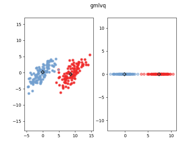
The following figure shows how GMLVQ classifies some example data after training. The blue dots show represent the prototype. The yellow and purple dots are the data points. The bigger transparent circle represent the target value and the smaller circle the predicted target value. The right side plot shows the data and prototypes multiplied with the learned $\Omega$ matrix. As can be seen, GMLVQ effectively projects the data onto a one-dimensinal line such that both classes are well distinguished. Note that this projection would not have been possible for GRLVQ because the relevant data direction is not parallel to a coordinate axis.

References:

[3]	“Adaptive Relevance Matrices in Learning Vector Quantization” Petra Schneider, Michael Biehl and Barbara Hammer - Neural Computation, vol. 21, nb. 12, pp. 3532-3561, 2009.

[4]	“Limited Rank Matrix Learning - Discriminative Dimension Reduction and Visualization” K. Bunte, P. Schneider, B. Hammer, F.-M. Schleif, T. Villmann and M. Biehl - Neural Networks, vol. 26, nb. 4, pp. 159-173, 2012.

Localized Generalized Matrix Learning Vector Quantization (LGMLVQ)¶

LgmlvqModel extends GLVQ by giving each prototype/class relevances for each feature. This way LGMLVQ is able to project the data for better classification.

Especially in multi-class data sets, the ideal projection $\Omega$ may be different for each class, or even each prototype. Localized Generalized Matrix Learning Vector Quantization (LGMLVQ) accounts for this locality dependence by learning an individual $\Omega_k$ for each prototype k [5]. As with GMLVQ, the rank of $\Omega$ can be bounded by using the dim parameter. After initializing the LgmlvqModel and calling the fit function on your data set, the learned $\Omega_k$ matrices can be retrieved via the attribute omegas_.

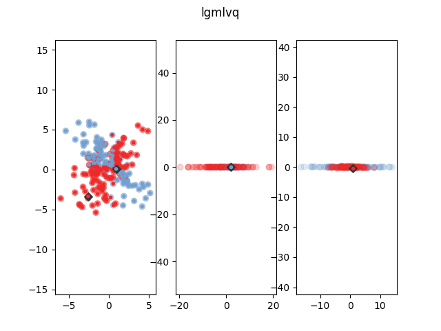
The following figure shows how LGMLVQ classifies some example data after training. The blue dots show represent the prototype. The yellow and purple dots are the data points. The bigger transparent circle represent the target value and the smaller circle the predicted target value. The plot in the middle and on the right show the data and prototypes after multiplication with the $\Omega_1$ and $\Omega_2$ matrix respectively. As can be seen, both prototypes project the data onto one dimension, but they choose orthogonal projection dimensions, such that the data of the respective own class is close while the other class gets dispersed, thereby enhancing classification accuracy. A GmlvqModel can not solve this classification problem, because no global $\Omega$ can enhance the classification significantly.

References:

[5]	“Adaptive Relevance Matrices in Learning Vector Quantization” Petra Schneider, Michael Biehl and Barbara Hammer - Neural Computation, vol. 21, nb. 12, pp. 3532-3561, 2009.

Implementation Details¶

This implementation is based upon the reference Matlab implementation provided by Biehl, Schneider and Bunte [6].

To optimize the GLVQ cost function with respect to all parameters (prototype positions as well as relevances and $\Omega$ matrices) we employ the LBFGS implementation of scipy. To prevent the degeneration of relevances in GMLVQ, we add the log-determinant of the relevance matrix $\Lambda = \Omega^T \cdot \Omega$ to the cost function, such that relevances can not degenerate to zero [7].

References:

[6]	LVQ Toolbox M. Biehl, P. Schneider and K. Bunte, 2017

[7]	“Regularization in Matrix Relevance Learning” P. Schneider, K. Bunte, B. Hammer and M. Biehl - IEEE Transactions on Neural Networks, vol. 21, nb. 5, pp. 831-840, 2010.